Load Balancing Algorithms
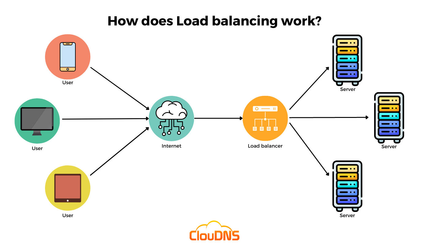
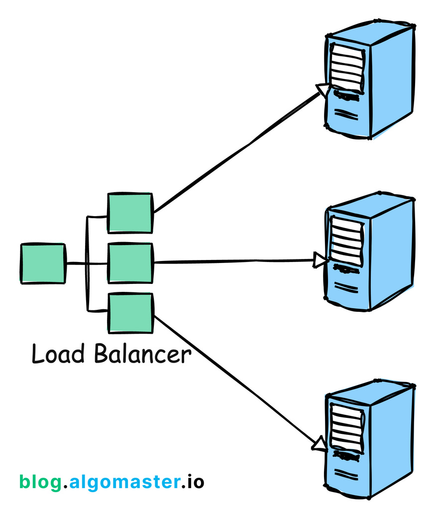
Load balancing is the process of distributing incoming network traffic across multiple servers to ensure that no single server is overwhelmed.
By evenly spreading the workload, load balancing aims to prevent overload on a single server, enhance performance by reducing response times and improve availability by rerouting traffic in case of server failures.
There are several algorithms to achieve load balancing, each with its pros and cons.
In this article, we will dive into the most commonly used load balancing algorithms, how they work, when to use them, their benefits/drawbacks and how to implement them in code.
Algorithm 1: Round Robin
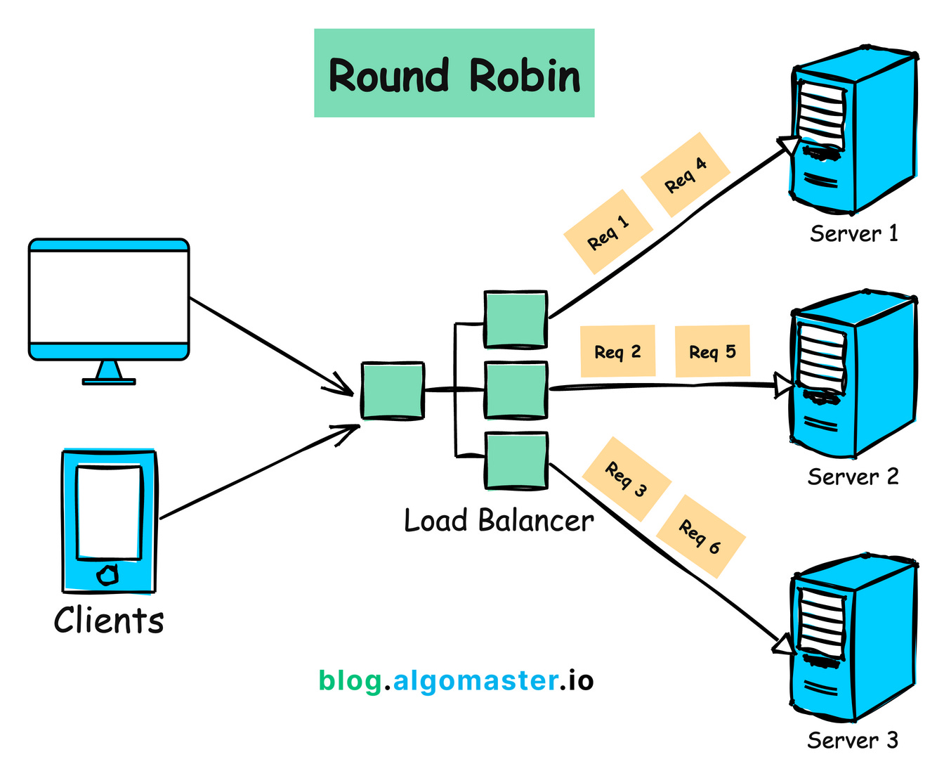
How it Works:
1.A request is sent to the first server in the list.
2. Next request is sent to the second server, and so on.
3.After the last server in the list, the algorithm loops back to the first server.
When to Use:
When all servers have similar processing capabilities and are equally capable of handling requests.
When simplicity and even distribution of load is more critical.
Benefits:
Simple to implement and understand.
Ensures even distribution of traffic.
Drawbacks:
Does not consider server load or response time.
Can lead to inefficiencies if servers have different processing capabilities.
Implementation:
class RoundRobin:

    def init(self, servers):

        self.servers = servers

        self.current_index = -1
    def get_next_server(self):
        self.current_index = (self.current_index + 1) % len(self.servers)
        return self.servers[self.current_index]

# Example usage
servers = ["Server1", "Server2", "Server3"]
load_balancer = RoundRobin(servers)


for i in range(6):
    server = load_balancer.get_next_server()
    print(f"Request {i + 1} -> {server}")
In this implementation, the RoundRobin class maintains a list of servers and keeps track of the current index.
The get_next_server() updates the index and returns the next server in the cycle.
Algorithm 2: Weighted Round Robin
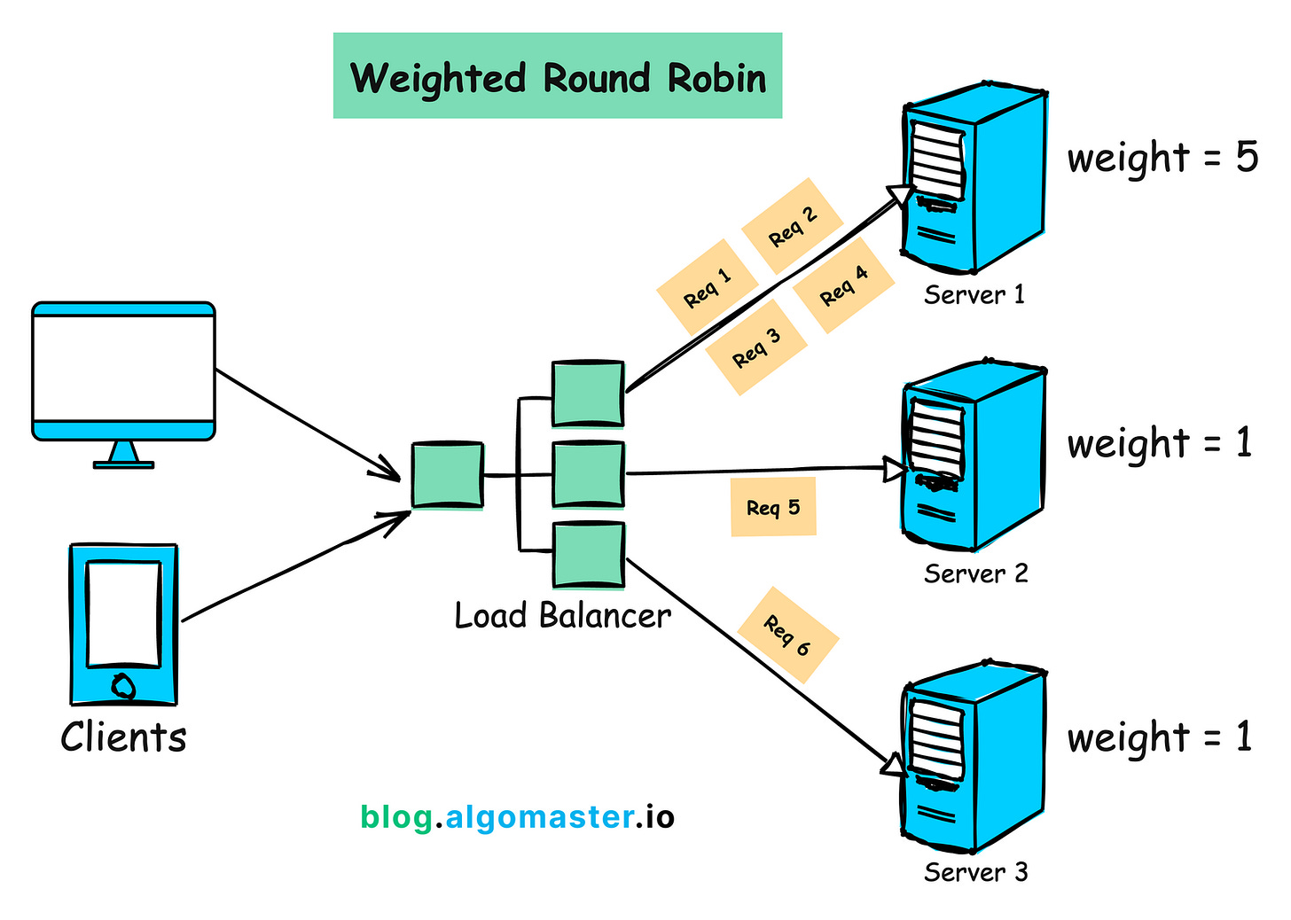
How it Works:
1.Each server is assigned a weight based on their processing power or available resources.
2.Servers with higher weights receive a proportionally larger share of incoming requests.
When to use:
When servers have different processing capabilities or available resources.
When you want to distribute the load based on the capacity of each server.
Benefits:
Balances load according to server capacity.
More efficient use of server resources.
Drawbacks:
Slightly more complex to implement than simple Round Robin.
Does not consider current server load or response time.
Implementation:
class WeightedRoundRobin:
    def init(self, servers, weights):
        self.servers = servers
        self.weights = weights
        self.current_index = -1
        self.current_weight = 0
    def get_next_server(self):
        while True:
            self.current_index = (self.current_index + 1) % len(self.servers)
            if self.current_index == 0:
                self.current_weight -= 1
                if self.current_weight <= 0:
                    self.current_weight = max(self.weights)
            if self.weights[self.current_index] >= self.current_weight:
                return self.servers[self.current_index]

# Example usage
servers = ["Server1", "Server2", "Server3"]
weights = [5, 1, 1]
load_balancer = WeightedRoundRobin(servers, weights)

for i in range(7):
    server = load_balancer.get_next_server()
    print(f"Request {i + 1} -> {server}")
In this implementation, the WeightedRoundRobin class takes a list of servers and their corresponding weights.
The get_next_server() method runs an infinite loop to find a suitable server based on the weights, ensuring that servers with higher weights receive more requests.
The algorithm keeps track of the current weight and adjusts it in each iteration to maintain the desired distribution ratio.
Example: if the weights are [5, 1, 1], Server 1 will be selected 5 times more often than Server 2 or Server 3.
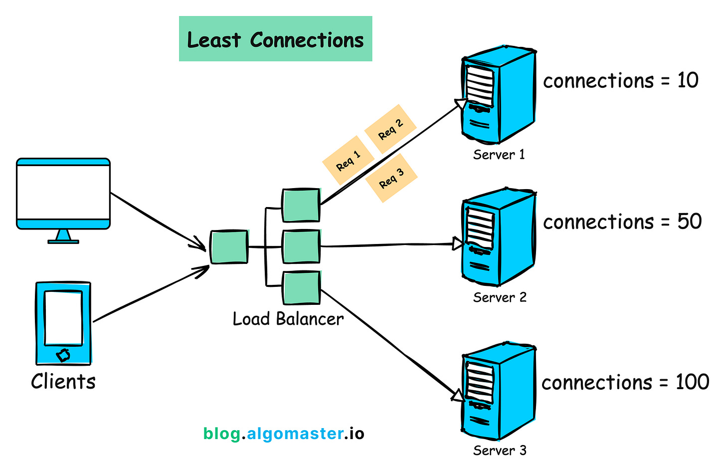
Algorithm 3: Least Connections
How it Works:
1.Monitor the number of active connections on each server.
2.Assigns incoming requests to the server with the least number of active connections.
When to use:
When you want to distribute the load based on the current number of active connections.
When servers have similar processing capabilities but may have different levels of concurrent connections.
Benefits:
Balances load more dynamically based on current server load.
Helps prevent any server from becoming overloaded with a high number of active connections.
Drawbacks:
May not be optimal if servers have different processing capabilities.
Requires tracking active connections for each server.
Implementation:
import random
class LeastConnections:
    def init(self, servers):
        self.servers = {server: 0 for server in servers}
    def get_next_server(self):
        # Find the minimum number of connections
        min_connections = min(self.servers.values())
        # Get all servers with the minimum number of connections
        least_loaded_servers = [server for server, connections in self.servers.items() if connections == min_connections]
        # Select a random server from the least loaded servers
        selected_server = random.choice(least_loaded_servers)
        self.servers[selected_server] += 1
        return selected_server

    def release_connection(self, server):
        if self.servers[server] > 0:
            self.servers[server] -= 1

# Example usage
servers = ["Server1", "Server2", "Server3"]
load_balancer = LeastConnections(servers)

for i in range(6):
    server = load_balancer.get_next_server()
    print(f"Request {i + 1} -> {server}")
    load_balancer.release_connection(server)
In this example, the LeastConnections class maintains a map of servers and the number of active connections for each server.
The get_next_server() method selects a random server with the least number of connections and increments the connection count for that server.
The release_connection() method is called when a connection is closed, decrementing the connection count for the corresponding server.
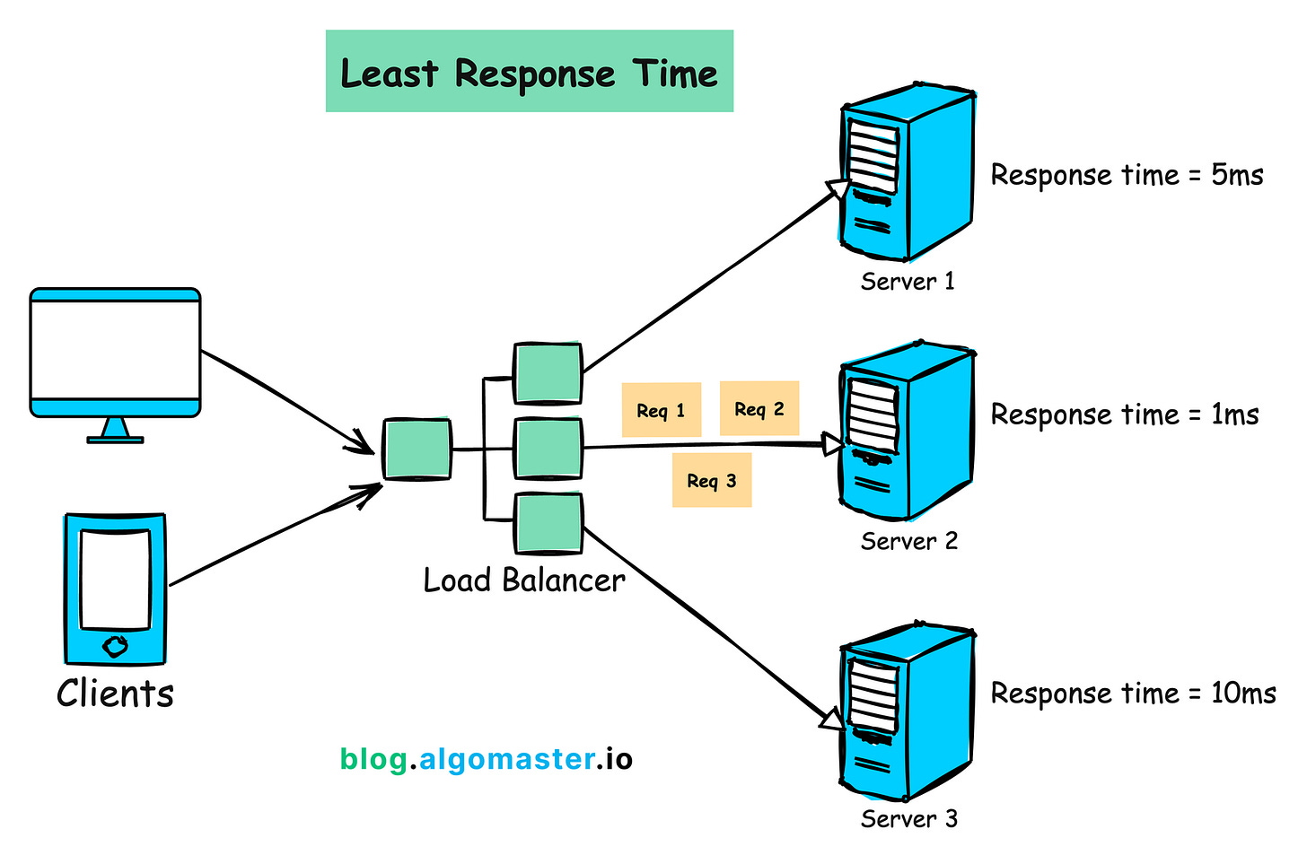
Algorithm 4: Least Response Time
How It Works:
Monitors the response time of each server
Assigns incoming requests to the server with the fastest response time.
When to Use:
- When you have servers with varying response times and want to route requests to the fastest server.
Benefits:
Minimizes overall latency by selecting the server with the fastest response time.
Can adapt dynamically to changes in server response times.
Helps improve the user experience by providing quick responses.
Drawbacks:
Requires accurate measurement of server response times, which can be challenging in distributed systems.
May not consider other factors such as server load or connection count.
Implementation:
import time
import random
class LeastResponseTime:
    def init(self, servers):
        self.servers = servers
        self.response_times = [0] * len(servers)

    def get_next_server(self):
        min_response_time = min(self.response_times)
        min_index = self.response_times.index(min_response_time)
        return self.servers[min_index]
    def update_response_time(self, server, response_time):
        index = self.servers.index(server)
        self.response_times[index] = response_time
# Simulated server response time function
def simulate_response_time():
    # Simulating response time with random delay
    delay = random.uniform(0.1, 1.0)
    time.sleep(delay)
    return delay

# Example usage
servers = ["Server1", "Server2", "Server3"]
load_balancer = LeastResponseTime(servers)

for i in range(6):
    server = load_balancer.get_next_server()
    print(f"Request {i + 1} -> {server}")
    response_time = simulate_response_time()
    load_balancer.update_response_time(server, response_time)
    print(f"Response Time: {response_time:.2f}s")
In this example, the LeastResponseTime class maintains a list of servers and keeps track of the response time for each server.
The get_next_server() method selects the server with the least response time. The update_response_time() method is called after each request to update the response time for the corresponding server.
To simulate the response time, we use a simulate_response_time() function that introduces a random delay to mimic the server's response time.
In a real-world scenario, you would measure the actual response time of each server.
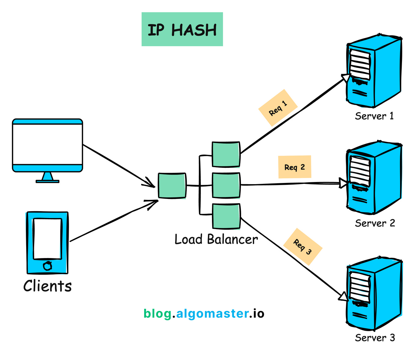
Algorithm 5: IP Hash
How It Works:
- Calculates a hash value from the client’s IP address and uses it to determine the server to route the request.
When to Use:
- When you need session persistence, as requests from the same client are always directed to the same server.
Benefits:
Simple to implement.
Useful for applications that require sticky sessions.
Drawbacks:
Can lead to uneven load distribution if certain IP addresses generate more traffic than others.
Lacks flexibility if a server goes down, as the hash mapping may need to be reconfigured.
Implementation:
import hashlib
class IPHash():
    def init(self, servers):
        self.servers = servers
    def get_next_server(self, client_ip):
        hash_value = hashlib.md5(client_ip.encode()).hexdigest()
        index = int(hash_value, 16) % len(self.servers)
        return self.servers[index]

# Example usage
servers = ["Server1", "Server2", "Server3"]
load_balancer = IPHash(servers)

client_ips = ["192.168.0.1", "192.168.0.2", "192.168.0.3", "192.168.0.4"]
for ip in client_ips:
    server = load_balancer.get_next_server(ip)
    print(f"Client {ip} -> {server}")
In this implementation, the IPHash class takes a list of servers.
The get_next_server() method calculates the MD5 hash of the client's IP address and uses the modulo operator to determine the index of the server to which the request should be routed.
This ensures that requests from the same IP address are always directed to the same server.
Summary:
Round Robin: Simple and even distribution, best for homogeneous servers.
Weighted Round Robin: Distributes based on server capacity, good for heterogeneous environments.
Least Connections: Dynamically balances based on load, ideal for varying workloads.
Least Response Time: Optimizes for fastest response, best for environments with varying server performance.
IP Hash: Ensures session persistence, useful for stateful applications.
Choosing the right load balancing algorithm depends on the specific needs and characteristics of your system, including server capabilities, workload distribution, and performance requirements.
